Core Machine Learning Algorithms

Now that we understand how machines learn, let's explore the core algorithms that make it all happen. While there are hundreds of different machine learning techniques, most fall into two fundamental categories based on what type of output they produce.

Regression algorithms predict continuous numerical values—like estimating house prices, forecasting temperatures, or predicting stock returns. Classification algorithms sort data into distinct categories—like identifying spam emails, diagnosing diseases, or recognizing objects in photos.

Regression: Predicting Numbers

Regression models excel at predicting continuous values where the output can be any number within a range. These algorithms learn relationships between input features and numerical outcomes.

🏠 House Price Prediction Example: We've seen this analogy a few times now, so why not use it again. This time, our model needs to consider multiple factors: house size, location quality, number of bedrooms, age of the property, and local market trends. Because we don't want to write out all these features (especially if we have more), we use the notation $1, ..., n$. This essentially means we start counting at 1 and end at $n$, the final number we have. Our formula remains in the same format though:

Let's break this down:

• $x_1, x_2, ..., x_n$ represent up to $n$ input features (size, location, ...).
• $w_1, w_2, ..., w_n$ are weights that determine how much each feature influences the price, $n$ corresponds to the number of input features.
• $b$ is the bias term that provides a baseline price estimate.

During training, the algorithm adjusts these weights to minimize prediction errors across thousands of house sales. Using this set up, we might get the following prediciton line:

Now, if we where to put a new house on the market that's 200m², we just check the prediction line and see that it's value could be about €125.000.

The beauty of regression is interpretability—you can see exactly how each feature contributes to the final prediction. If the location weight is large and positive, it means good locations significantly increase house values.

Classification: Sorting into Categories

Classification algorithms predict discrete categories or labels rather than continuous numbers. The output is always one of a predefined set of classes.

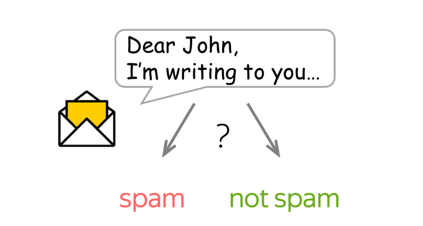
📧 Email Spam Detection Example: When your email provider analyzes an incoming message, it needs to decide: spam or legitimate? This is called a binary classification problem because there are only two possible outcomes.

Image Creds

The algorithm looks at various features of the email—certain keywords, sender reputation, message length, number of exclamation points—and combines all this information to make a decision. Instead of giving a simple yes/no answer, many classification algorithms provide a confidence score.

Classification isn't limited to two categories, when more classes are involved we can use Multi-class Classification. An image recognition system might classify photos into dozens of categories: cat, dog, car, tree, person, etc. The same principles apply, but the algorithm outputs probabilities for each possible class.

From Simple to Complex Relationships

The linear models we have seen so far represent the simplest and most interpretable approach to machine learning. They assume relationships between inputs and outputs can be captured with straight lines.

👩🏻‍🏫 Predicting Exam Scores Example: Let's dive into a new example, suppose we want to predict student exam scores based on study hours. If there's a consistent relationship—more study time leads to better scores—linear regression can capture this pattern:

This line would look very similar to the plot showing linear regression earlier in this chapter. However, not all relationships are linear, many times in fact we need a more complex function to model relationships.

Modeling Non-Linear Relationships

Real-world relationships are often not straight lines. House prices might increase slowly for small homes, then rapidly for larger ones, creating a curved relationship. This is where we diverge to something called "Polynomial Regression".

🏠 House Price Prediction Example: Instead of modeling a straight line, this time we will use polynomial regression to introduce curved relationships by adding higher-degree terms:

By including quadratic or cubic terms, the model can fit curved patterns in the data. Notice how this fit is better suited for the housing data than our linear fit from before.

The polynomial model can capture more complex patterns, but it's also more prone to overfitting—especially with higher-degree terms.

Prediction Models: Learning from Probability

While linear regression models relationships between numerical variables, and classification models separate data into categories, some models approach prediction using probability theory. These models are particularly useful when dealing with uncertainty in data.

Naïve Bayes: Classification Through Probability

Naive Bayes applies Bayes' Theorem, which we lightly referred to in Chapter 2, to classification problems. Despite its "naive" assumption that all features are independent, it works remarkably well for many real-world tasks.

Mathematically, Bayes' Theorem states:

Let's break this down:

• $P(\text{class} | \text{features})$: probability of a certain class given the input features.
• $P(\text{features} | \text{class})$: probability of observing those features if the class is known.
• $P(\text{class})$: prior probability of that class occurring (e.g., the chance of heads in a coin flip is 50%).
• $P(\text{features})$: overall probability of observing those features (used to normalize the result and often omitted).

📧 Spam Detection Example: Let’s say an email contains the phrase “free money” and comes from an unknown sender. We break the problem into parts:

• $P(\text{spam}) = 0.3$ (30% of all emails in our dataset are spam — the prior).
• $P(\text{``free money"} | \text{spam}) = 0.8$ (“free money” appears in 80% of spam emails).
• $P(\text{unknown sender} | \text{spam}) = 0.6$ (60% of spam emails come from unknown senders).

The model combines these individual probabilities to make a final classification decision:

This product gives us an unnormalized score for the spam class. We’d do the same for the not spam class and then compare both to decide which is more likely.

The term "naïve" is used because the algorithm assumes that knowing one feature doesn't give you information about others. In reality, email features are often related—emails with "free" often also contain "money" or exclamation points. Despite this oversimplification, Naive Bayes is fast, effective, and widely used for text classification, medical diagnosis, and sentiment analysis.

Gradient Descent: How AI Actually Learns

Throughout this chapter, we've mentioned that models "adjust weights to minimize errors," but how does this actually happen? The answer is gradient descent—a mathematical optimization technique that uses derivatives (from Chapter 2) to systematically improve model performance.

⛰ Hill-Climbing Example: Imagine you're blindfolded on a hilly landscape, trying to reach the lowest valley (minimum error). Gradient descent is like feeling the slope under your feet and always taking a step in the steepest downhill direction. Eventually, you'll reach a valley—hopefully the lowest one.

Remember our house price prediction model:

Gradient descent adjusts the weights $w_1, w_2$ and bias $b$ using this process:

1. Calculate the error: How far off are our current predictions?
2. Find the gradient: Use derivatives to determine which direction to adjust each weight.
3. Take a step: Move weights slightly in the direction that reduces error.
4. Repeat: Continue until the error stops improving.

This is where derivatives from Chapter 2 become crucial. The gradient tells us:

• If increasing $w_1$ would increase or decrease the error.
• How much to change $w_2$ for maximum improvement.
• The same for $w_2$, $b$, and any other parameters.

The learning rate determines how big steps to take. Too large, and you might overshoot the minimum and bounce around wildly. Too small, and learning takes forever. Finding the right learning rate is part of the art of machine learning.

Gradient descent is the engine that powers most machine learning algorithms. Whether you're training a simple linear regression or a complex neural network, this same principle—use derivatives to systematically reduce errors—drives the learning process.

Clustering: Finding Hidden Groups

Unlike supervised algorithms that learn from labeled examples, clustering algorithms discover hidden patterns in unlabeled data.

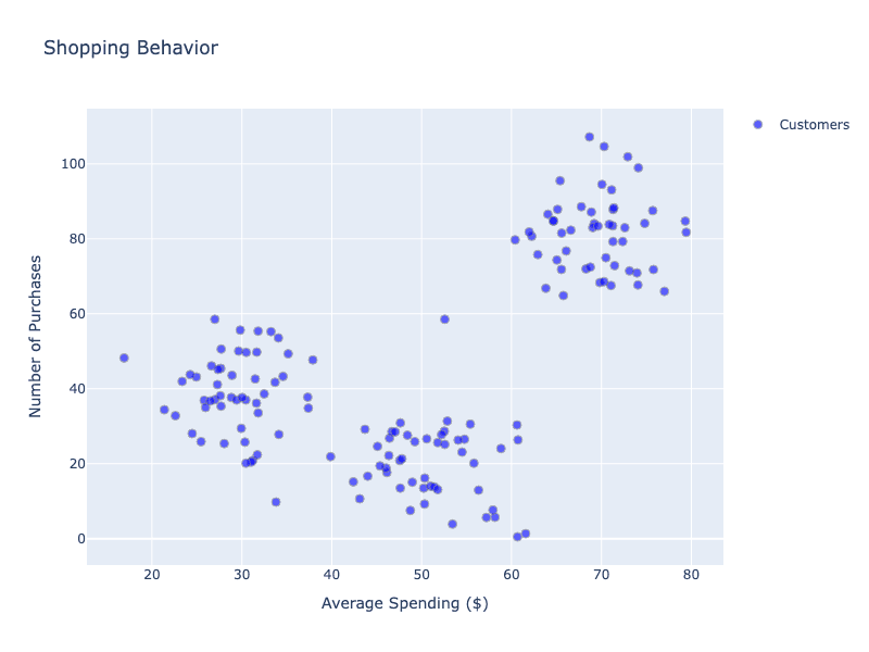
K-Means Clustering: We've seen this case before, an e-commerce company wants to understand their customer base without predefined categories. K-Means groups customers based on shopping behavior similarities:

Clearly, we see a pattern emerging again. In several steps, K-Means automatically groups data based on feature similarity:

1. Choose the number of clusters (k).
2. Place cluster centers randomly.
3. Assign each customer to the nearest center.
4. Move centers to the average position of assigned customers.
5. Repeat until centers stabilize.

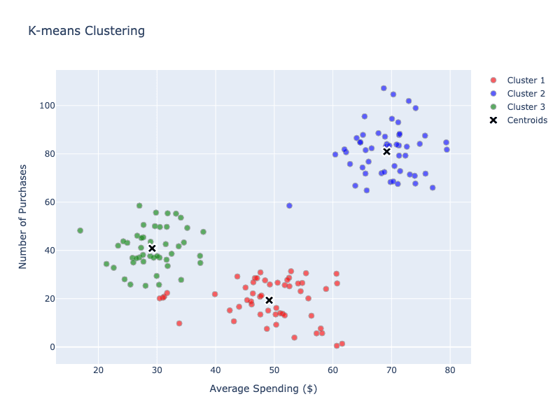
After a few iterations, using a K-means algorithm, we have defined "centroids", centralized points that define groups, or clusters:

The algorithm might have discovered natural customer segments:

• Budget Conscious: Low spending, high frequency.
• Premium Buyers: High spending, low frequency.
• Occasional Shoppers: Medium spending, irregular timing.

K-means is a solid technique used in many applications like market segmentation for targeted marketing or image segmentation in computer vision.

Dimensionality Reduction: Simplifying Data

Real-world datasets often have too many features to analyze or visualize directly. Principal Component Analysis (PCA) reduces this complexity by projecting data onto the directions of greatest variation—like choosing the best camera angles to capture a 3D object’s shape.

🫥 Face Recognition Example: Instead of analyzing every pixel in a face photo (potentially thousands of features), PCA identifies the most important facial variations—overall face shape, eye position, nose structure. This reduces computational requirements while maintaining recognition accuracy.

Some other benefits of Dimensionality Reduction:

• Faster training and prediction.
• Reduced storage requirements.
• Easier data visualization.

Reducing dimensions always involves some information loss. The key is finding the right balance between simplification and maintaining essential patterns.

Choosing the Right Algorithm

This chapter is meant to give you a brief overview of techniques. Note that there are many more techniques or variants on techniques out there. Selecting the appropriate algorithm depends on several factors:

Problem Type:

• Predicting numbers? Use regression (linear, polynomial, or more complex variants).
• Categorizing data? Use classification (logistic regression, Naive Bayes, or others).
• Finding patterns? Use clustering or dimensionality reduction.

Data Characteristics:

• Small datasets: Simple models like linear regression often work best.
• Large datasets: More complex models can capture subtle patterns.
• Many features: Consider dimensionality reduction first.
• Text data: Naive Bayes is often a good starting point.

Interpretability Requirements:

• Need to explain decisions? Linear models provide clear feature importance.
• Black box acceptable? More complex models might achieve higher accuracy.

Choosing which machine learning technique to use is an important step in modeling any system, including AI.

Final Takeaways

Machine learning algorithms fall into clear categories based on their purpose and approach. Regression algorithms predict continuous values using mathematical relationships between features and outcomes. Classification algorithms sort data into categories using probability or decision boundaries. Clustering algorithms find hidden patterns in unlabeled data. Each approach has specific strengths and ideal use cases, and understanding these fundamentals helps you choose the right tool for any machine learning problem you encounter.